Retail Demand Forecasting with Graph Neural Networks: Mathematical Principles, Controlled Experiments, and Production Boundaries

Table of Contents
At 10 a.m. on a Friday, a neighbourhood store of a supermarket chain is suddenly packed with shoppers. Watching a long line form in front of the chilled display cases, the store manager is baffled: today is not a public holiday, the store is running no discounts or promotions, and the backend single-store forecasting system recommended only normal everyday stock yesterday—where did this sudden rush come from?
The answer does not lie in this store’s own historical sales ledger. It lies two kilometers down the street in the same commercial district: a sister store down the block launched a major promotion this morning, but the eastern regional warehouse supplying that neighbour suffered a sorting breakdown the night before, leaving its shelves empty shortly after opening. Shoppers drawn into the district by the promotion came away empty-handed and walked down the street to this store, which receives normal replenishment from the western regional warehouse.
Our earlier articles on Prophet and tree models largely assumed that a store’s future is governed by its own past. In a retail network, neighbouring stores can move traffic in opposite directions:
- Promotional cannibalization: a well-stocked neighbour runs a deep discount and draws away price-sensitive shoppers.
- Stockout spillover: the promoted neighbour sells out, so unmet demand moves to another store.
Once we step into a retail network like this, any forecasting method that looks only at a single store’s own history suffers from a structural information blind spot. Forecasting is no longer a matter of extrapolating an isolated time series; it must answer two intertwined questions at once: How do warehouse and store states evolve over time, and how do supply conditions and customer-flow signals propagate across the warehouse–store network?
This is where stochastic processes and graph neural networks (GNNs) meet: one describes how states evolve; the other learns how information moves through supply and spatial relationships. The real question is not whether a GNN is more advanced, but whether an improvement came from cleaner observations, genuinely new information, or greater model capacity. The article follows that chain from mechanism to controlled evidence and then to production boundaries.
Results at a glance
- Repairing stockout censoring reduces overall WAPE from 18.14% to 13.78%, without a graph model.
- One-hop tree models reduce spillover-period WAPE from roughly 22% to 10.38%–10.90%.
- Under strong controlled coupling, the neural heterogeneous GNN reaches 3.26% spillover-period WAPE (the contributions of graph structure and continuous nonlinearity have not been separated). With zero coupling, it scores 4.21%, worse than the local model’s 3.06%.
- On all three public panels, the graph-aggregated ridge model fails to beat the best non-graph baseline. It is not the neural GNN used in the controlled experiment.
The companion data generator, public-data loaders, model comparisons, and complete experiment records are open-sourced at GitHub: retail-gnn-demand-forecast.
1. How Do Stochastic Processes Characterize Temporal State Evolution? #
Before choosing a forecasting method, we should ask what the observed sales, inventory, and supply states really are: static numbers, or traces left by a changing system? Retail demand moves with calendars and promotions, while warehouses switch among normal, congested, and disrupted operation. The value of stochastic processes lies not only in their probability formulas, but in the discipline of defining the state, how it changes, and which changes remain uncertain. Relationships between entities have a sound foundation only after temporal evolution is clear.
1.1 Stochastic Processes, the Markov Property, and Transition Matrices #
A stochastic process is a family of random variables indexed by time or another parameter:
\[ \{X_t:t\in T\} \]Here, \(T\) is the index set, usually time but sometimes space or another ordered dimension. The variable \(X_t\) may be a discrete state, continuous value, or vector. The definition requires neither the Markov property nor a stationary distribution.
Adopting a discrete-time Markov chain further assumes that a well-designed current state already contains the historical information needed to predict the next step:
\[ \Pr(X_{t+1}\mid X_t,X_{t-1},\ldots,X_0)=\Pr(X_{t+1}\mid X_t) \]This is the Markov property (often called memorylessness). It does not claim that earlier history has no business value; rather, it requires the model’s defined “current state” to already summarize the relevant history. If the next step still depends on how long a state has lasted or on its recent trajectory, that information should be incorporated into the state definition or modelled with a higher-order process.
For a finite state space \(\mathcal S=\{s_1,s_2,\ldots,s_m\}\), a row-stochastic matrix \(\mathbf P\), or state transition matrix, represents one-step transitions. Its entries are non-negative probabilities and each row sums to \(1\):
\[ \begin{aligned} P_{ab}&=\Pr(X_{t+1}=s_b\mid X_t=s_a),\\ \boldsymbol\pi_{t+1}&=\boldsymbol\pi_t\mathbf P,\\ \boldsymbol\pi_{t+k}&=\boldsymbol\pi_t\mathbf P^k. \end{aligned} \]Here, \(\boldsymbol\pi_t\) is the state probability distribution at time \(t\). If \(\mathbf P\) does not change with calendar time, the chain is time-homogeneous, and \(\mathbf P^k\) gives the distribution after \(k\) steps. Real applications must still estimate the transition probabilities and test this assumption.
1.2 “Stationary” Does Not Mean “Unchanging” #
Weak stationarity in time-series analysis asks whether the mean, variance, and autocovariance change with calendar time. A Markov chain’s stationary distribution asks a different question: when the same transition rule is applied repeatedly, what long-run proportion of time does the system spend in each state? Retail sales often violate the first condition because of trends, seasons, and promotions, while warehouse states may still settle into long-run proportions under a fixed transition rule:
\[ \boldsymbol\pi^*=\boldsymbol\pi^*\mathbf P \]When the chain satisfies the relevant convergence conditions, \(\boldsymbol\pi^*\) describes the long-run proportions of normal, congested, and disrupted warehouse operation. A spatial graph may also use a row-normalized matrix, but its entries are aggregation or allocation weights—not warehouse-state probabilities and not automatically observed shopper-transition probabilities. Similar matrix forms do not give the two objects the same business meaning.
2. How Graph Neural Networks Learn from Entity Relationships #
Chapter 1 treated the forecast target as a state that evolves over time. Chapter 2 asks a further question: is an entity’s future determined only by itself? The first value of a graph is not a new model; it is the discipline of stating who may affect whom, which relationship carries the information, and whether different relationships deserve different rules. In retail, one product may sit across many stores, one warehouse may supply several districts, and a promotion or stockout may alter traffic at neighbouring stores. Connecting these entities is meaningful only when the relationships have a defensible business interpretation.
Suppose we want to forecast tomorrow’s product demand at a specific store. A traditional single-store time-series model predicts from that store’s own sales history, prices, holidays, and promotions; yet if a nearby store runs a major promotion, or stocks out after an upstream warehouse delay, shoppers may switch stores. A single store’s own historical series cannot fully capture these cross-store shifts. The forecasting problem therefore changes: a system’s state depends not only on its own history, but also on connected entities.
2.1 Understanding Graph Structure Through a Minimal Retail Network #
To avoid switching scenarios across formulas, this chapter tracks one local network: warehouse \(W_1\) supplies store \(S_1\), warehouse \(W_2\) supplies store \(S_2\), and the two stores can influence each other’s customer traffic. Our task is to jointly predict next-day demand at \(S_1\) and \(S_2\).
A graph represents business entities as nodes and relationships between entities as edges. Write a graph as \(G=(\mathcal V,\mathcal E)\), where \(\mathcal V\) is the node set and \(\mathcal E\) is the edge set. This four-node teaching subgraph is:
\[ \begin{aligned} \mathcal V&=\{W_1,W_2,S_1,S_2\},\\ \mathcal E&=\{(W_1,S_1),(W_2,S_2),(S_2,S_1),(S_1,S_2)\}. \end{aligned} \]Here, \(W_1,W_2\) are warehouse nodes and \(S_1,S_2\) are store nodes. Edges \((W_1,S_1)\) and \((W_2,S_2)\) represent supply relationships, while the spatial relationship between the two stores expands into two directed edges, \((S_1,S_2)\) and \((S_2,S_1)\). In compact arrow notation:
\[ W_1\overset{\mathrm{sup}}{\longrightarrow}S_1 \overset{\mathrm{spa}}{\longleftrightarrow}S_2 \overset{\mathrm{sup}}{\longleftarrow}W_2 \]Above the arrows, \(\mathrm{sup}\) denotes a supply relationship and \(\mathrm{spa}\) denotes a spatial relationship. Arrow direction indicates that information can flow from the source node to the target node: supply information flows from warehouse to store, whereas the spatial relationship uses both directions so that either store’s information can inform the other’s forecast.
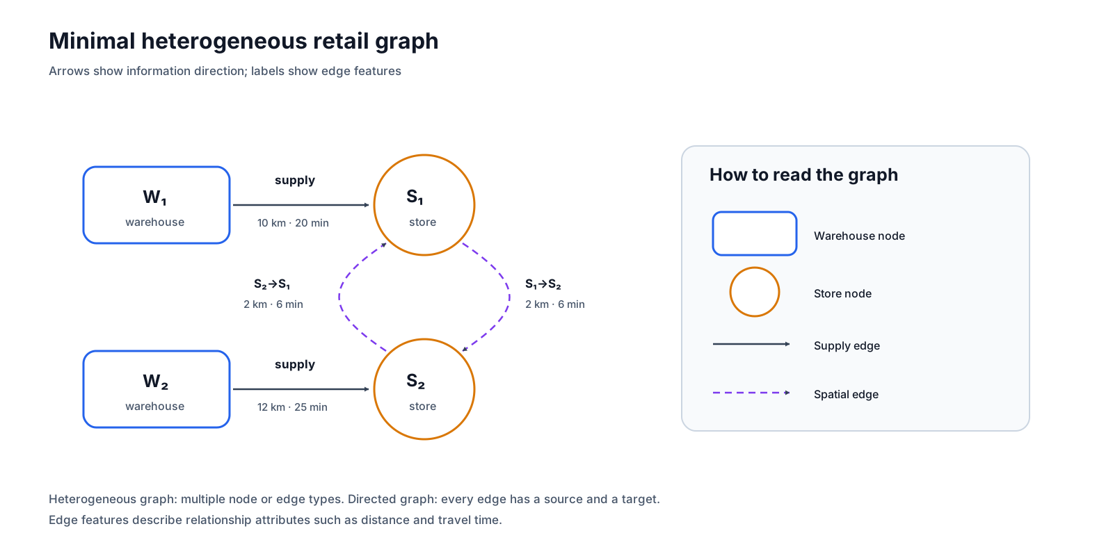
Because these edges distinguish source from target, this is a directed graph. For example, \(W_1\to S_1\) allows supply information to flow only from warehouse \(W_1\) to store \(S_1\), while \(S_2\to S_1\) allows the state of \(S_2\) to inform the forecast for \(S_1\). Direction specifies which entity’s information may update another entity; it does not represent a fixed direction of physical customer movement or predetermine whether demand increases or decreases.
Because this example includes two node types (warehouses and stores) and two edge types (supply and spatial), it forms a heterogeneous graph. A graph with one node type and one edge type is homogeneous.
Distance and travel time are edge features that describe a relationship. Assigning each edge a scalar strength \(w_e\) yields a weighted graph; “weight” usually means the scalar used in aggregation.
Finally, an edge in a graph only records a relationship that the model is allowed to use; it does not automatically prove causality. When \(S_2\) runs a promotion with ample stock, it may draw traffic away from \(S_1\); when \(S_2\) stocks out during a promotion, the same spatial connection may spill unmet demand over to \(S_1\). Graph topology answers which entities are linked; the direction and magnitude of a given day’s impact depend on the current states of the nodes and edges.
2.2 How Do We Represent Graph Structure and Business State as Data? #
The graph \(G\) specifies which entities are connected. The model also needs the node states and relationship attributes on date \(t\). A heterogeneous graph does not have to pad different entities into one matrix; warehouses, stores, supply edges, and spatial edges can each retain fields suited to their roles:
| Object | Teaching data on date \(t\) | What the model can read |
|---|---|---|
| Warehouses \(W_1,W_2\) | Supply availability \(1,0\) | Which warehouse can supply normally |
| Stores \(S_1,S_2\) | Recent demand \(100,80\); promotion \(0,1\) | Local demand and promotion state |
| Supply edges | Distance \(10,12\) km; travel time \(20,25\) min | Warehouse-to-store relationship attributes |
| Spatial edges | Distance \(2\) km; travel time \(6\) min | Strength and direction of the store relationship |
Let \(\mathbf X_t^{\mathrm W}\) and \(\mathbf X_t^{\mathrm S}\) denote warehouse and store features, and let \(\mathbf R_t^{\mathrm{sup}}\) and \(\mathbf R_t^{\mathrm{spa}}\) denote the two edge-feature sets. The complete snapshot for one date is
\[ \mathbf z_t=\left(G,\{\mathbf X_t^{\mathrm W},\mathbf X_t^{\mathrm S}\}, \{\mathbf R_t^{\mathrm{sup}},\mathbf R_t^{\mathrm{spa}}\}\right). \]A fixed topology can be stored separately, while changing states are recorded by date and entity. To keep the calculation in Section 2.4 transparent, the example uses only supply availability, demand, and promotion. Distance and travel time remain valid edge features for a production model. All values are teaching assumptions, not industry averages.
2.3 How Do We Define and Train a GNN Forecasting Task? #
Write the complete GNN as \(f_\Theta\). It reads the graph snapshot on date \(t\) and jointly predicts next-day demand at the two stores:
\[ \widehat{\mathbf y}_{t+1}= \begin{bmatrix} \hat y_{S_1,t+1}\\ \hat y_{S_2,t+1} \end{bmatrix}=f_\Theta(\mathbf z_t). \]Each historical date creates one dated-input and next-day-label pair. Let \(\mathcal T_{\mathrm{train}}\) be the training dates, \(\mathcal D_{\mathrm{train}}\) the corresponding samples, and \(y^{\mathrm{target}}\) the next-day label. With mean squared error, the model learns \(\Theta\) by minimizing error across all training dates and target stores:
\[ \Theta^*=\underset{\Theta}{\operatorname{argmin}}\; \frac{1}{|\mathcal D_{\mathrm{train}}|\,|\mathcal V^{\mathrm S}|} \sum_{t\in\mathcal T_{\mathrm{train}}} \sum_{S_i\in\mathcal V^{\mathrm S}} \left(y_{S_i,t+1}^{\mathrm{target}}-\hat y_{S_i,t+1}\right)^2. \]The crucial issue is not the loss function but the label. Sales censoring means that if only 50 units are in stock, the till can record at most 50 sales even when customers want 80. A latent-demand target therefore requires stockout filtering, reconstruction, or an explicit censored model. A GNN can propagate information, but it cannot automatically repair a biased label.
2.4 How Does Message Passing Turn Graph Data into a Forecast? #
After defining the input, output, and training target, we can inspect how \(f_\Theta\) makes one prediction. A message passing neural network (MPNN) generates messages from the edge type and endpoint states, aggregates messages that reach the same node, updates the node representation, and converts the result into a forecast.
The diagram shows the full chain first: warehouse states enter store representations, the stores exchange spatial messages, and a shared prediction head produces next-day demand.
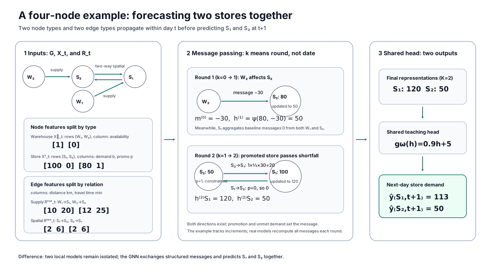
Numerical Example: How Does the Four-Node Network Produce a Forecast? #
Return to the four-node network and follow one inference pass after training. Section 2.3 learns \(\Theta\) from many dated input-label pairs. Here the parameters are fixed, and a new snapshot on date \(t\) is converted into a forecast for date \(t+1\). The values \(-30\), \(2/3\), \(0.9\), and \(5\) are chosen only to make the arithmetic easy to verify. They are not fitted from the few values shown above and are not empirical retail coefficients.
Node representations \(\mathbf h_{S_i,t}^{(k)}\) are usually vectors. This example reduces them to scalars \(h_{S_i}^{(k)}\) and suppresses their shared date subscript. Recent demand initializes the stores: \(h_{S_1}^{(0)}=100\) and \(h_{S_2}^{(0)}=80\). The same snapshot gives \(a_{W_1,t}^{\mathrm W}=1\), \(a_{W_2,t}^{\mathrm W}=0\), \(p_{S_1,t}=0\), and \(p_{S_2,t}=1\). The graph and its dated features remain fixed throughout the calculation. Superscripts \((0)\), \((1)\), and \((2)\) mark the initial representation and two propagation rounds within the same snapshot; they do not advance the calendar to \(t+2\).
One propagation along an edge is one hop. Round 1 lets each store receive warehouse information, and Round 2 lets the stores exchange their updated information. The path \(W_2\to S_2\to S_1\) therefore spans two hops. Propagation depth describes the information range within one dated snapshot, not two days of elapsed time.
The general functions now become four rules that we can calculate by hand. A full model would encode warehouse features into a warehouse representation \(\mathbf h_W\). This example lets the supply message read warehouse availability \(a^{\mathrm W}\) directly. The spatial message reads source-store demand \(b_{S_j,t}\), promotion \(p_{S_j,t}\), and the Round-1 representation \(h_{S_j}^{(1)}\). Distance and travel time remain in \(\mathbf R_t\) but do not enter this calculation.
| Component | Inputs | Simplified rule |
|---|---|---|
| Supply message \(\phi^{\mathrm{sup}}\) | \(a_{W_j,t}^{\mathrm W}\) | \(m_{W_j\to S_i,t}^{(0),\mathrm{sup}}=-30(1-a_{W_j,t}^{\mathrm W})\) |
| Spatial message \(\phi^{\mathrm{spa}}\) | \(b_{S_j,t},\,p_{S_j,t},\,h_{S_j}^{(1)}\) | \(m_{S_j\to S_i,t}^{(1),\mathrm{spa}}=p_{S_j,t}\frac{2}{3}\max(0,b_{S_j,t}-h_{S_j}^{(1)})\) |
| Update function \(\psi\) | \(h_{\mathrm{old}},\,m\) | \(h_{\mathrm{new}}=h_{\mathrm{old}}+m\) |
| Prediction head \(g_\omega\) | \(h_{S_i}^{(2)}\) | \(\hat y=g_\omega(h)=0.9h+5\) |
Message subscripts identify the directed edge. Superscripts \((0)\) and \((1)\) show whether a message uses the initial or Round-1 representation, while \(\mathrm{sup}\) and \(\mathrm{spa}\) distinguish supply and spatial messages. In the teaching prediction head, \(\omega\) contains the slope \(0.9\) and intercept \(5\). Production functions are usually richer; these rules only expose one forward pass.
Write the full two-store forecast first:
\[ \begin{aligned} \widehat{\mathbf y}_{t+1} &= \begin{bmatrix} \hat y_{S_1,t+1}\\ \hat y_{S_2,t+1} \end{bmatrix} = \begin{bmatrix} 0.9h_{S_1}^{(2)}+5\\ 0.9h_{S_2}^{(2)}+5 \end{bmatrix} = \begin{bmatrix} 0.9\times120+5\\ 0.9\times50+5 \end{bmatrix} = \begin{bmatrix} 113\\ 50 \end{bmatrix}. \end{aligned} \]The values \(120\) and \(50\) come from the two rounds below.
Round 1: Supply messages update store representations. When \(a^{\mathrm W}=1\), the warehouse supplies normally and sends 0. When \(a^{\mathrm W}=0\), it sends \(-30\). Warehouse \(W_1\) therefore leaves \(S_1\) unchanged, while unavailable \(W_2\) changes \(S_2\) from 80 to 50:
\[ \begin{aligned} m_{W_1\to S_1,t}^{(0),\mathrm{sup}} &= -30(1-1)=0,\\ m_{W_2\to S_2,t}^{(0),\mathrm{sup}} &= -30(1-0)=-30,\\[4pt] h_{S_1}^{(1)} &= 100+m_{W_1\to S_1,t}^{(0),\mathrm{sup}}=100,\\ h_{S_2}^{(1)} &= 80+m_{W_2\to S_2,t}^{(0),\mathrm{sup}}=50. \end{aligned} \]The value \(-30\) only illustrates how constrained supply changes an internal representation. It does not mean real demand must fall by 30 units.
Round 2: Spatial messages transmit the supply effect to the neighbour. The spatial function computes the source store’s shortfall \(b_{S_j,t}-h_{S_j}^{(1)}\), then uses promotion \(p_{S_j,t}\) as a gate. When \(p=0\), the message is 0. When \(p=1\), this rule passes two-thirds of the shortfall to the neighbour. Promoted store \(S_2\) has a shortfall of \(80-50=30\), so it sends 20 to \(S_1\). Unpromoted \(S_1\) sends 0 to \(S_2\):
\[ \begin{aligned} m_{S_2\to S_1,t}^{(1),\mathrm{spa}} &= 1\times\frac{2}{3}(80-50)=20,\\ m_{S_1\to S_2,t}^{(1),\mathrm{spa}} &= 0\times\frac{2}{3}\max(0,100-100)=0,\\[4pt] h_{S_1}^{(2)} &= 100+m_{S_2\to S_1,t}^{(1),\mathrm{spa}}=120,\\ h_{S_2}^{(2)} &= 50+m_{S_1\to S_2,t}^{(1),\mathrm{spa}}=50. \end{aligned} \]The prediction head reads \(h_{S_1}^{(2)}=120\) and \(h_{S_2}^{(2)}=50\) and outputs 113 and 50. The spatial message of 20 is an internal demand-transfer signal, not a final forecast or a claim that exactly 20 shoppers or orders moved.
Abstracting the example back to a general MPNN, \(\phi^r\) generates messages for relation type \(r\), \(\operatorname{AGG}\) combines messages arriving at one node, \(\psi\) updates its representation, and the prediction head \(g_\omega\) produces the output[1]:
\[ \begin{aligned} \mathbf m_{i,t}^{(k),r} &=\operatorname{AGG}\Bigl\{\phi^r(\mathbf h_{j,t}^{(k)},\mathbf r_{j\to i,t})\\ &\qquad\bigm| j\to i\in\mathcal E^r\Bigr\},\\ \mathbf h_{i,t}^{(k+1)} &=\psi(\mathbf h_{i,t}^{(k)},\{\mathbf m_{i,t}^{(k),r}\}_r), \qquad \hat y_{i,t+1}=g_\omega(\mathbf h_{i,t}^{(K)}). \end{aligned} \]What Characteristics of a GNN Does This Example Illustrate? #
The example is about more than adding columns. It shows how fields participate in computation through graph structure:
- The graph constrains where information can travel. Supply status at \(W_2\) enters \(S_2\) along a supply edge and then reaches \(S_1\) along a spatial edge. Remove either \(W_2\to S_2\) or \(S_2\to S_1\), and the two-hop path disappears.
- Multiple rounds compose different relationship types. Round 1 writes supply availability into the store representation. Round 2 computes a cross-store message from demand, promotion, and that updated state. The forecast for \(S_1\) therefore combines its local signal with “upstream supply constraint plus neighbour promotion.”
- Relationships of the same type share a rule. Both warehouse-to-store edges use the supply message function, and both store-to-store edges use the spatial message function. A larger network can reuse these relation-specific rules instead of fitting separate parameters for every node.
Ordinary models can also use neighbourhood fields. Engineers can flatten them into a wide table for a linear model, tree model, or multilayer perceptron. A GNN instead encodes who can send which type of information to whom and shares the rule across edges of the same type. Whether that structure performs better still requires strict out-of-time testing.
2.5 How Do GCN, GraphSAGE, and GAT Aggregate Neighbours Differently? #
GCN, GraphSAGE, and GAT all follow the message-passing framework. Their main difference is which neighbours they read and how they summarize them[2][3][4]. Classical versions assume compatible node representations. Because warehouses and stores have different fields here, a practical model first projects each type into a shared hidden space:
\[ \mathbf H_{\mathrm W}^{(0)}=f_{\mathrm W}(\mathbf X_t^{\mathrm W}), \qquad \mathbf H_{\mathrm S}^{(0)}=f_{\mathrm S}(\mathbf X_t^{\mathrm S}). \]Supply and spatial edges carry different business meanings, so they should not automatically share message parameters even after their endpoint representations have compatible dimensions.
| Model | Neighbours used per round | How the summary is formed | Main consideration |
|---|---|---|---|
| GCN | Usually the complete one-hop neighbourhood | Normalize by topology and node degree | Simple structure and a useful introductory graph baseline |
| GraphSAGE | Can sample a fixed number of neighbours | Shared mean, pooling, or learned aggregator | Controls computation on large graphs and supports inductive use on new nodes |
| GAT | Usually the target node’s current neighbourhood | Learn attention weights from current representations | More flexible when neighbour influence changes with input state |
These models are not a performance hierarchy. The choice depends on graph scale, whether new nodes must be handled, and whether neighbour influence varies with state. Attention weights describe how one aggregation step allocates weight; they do not prove causality. A heterogeneous directed retail graph must still preserve edge direction and use different rules for supply and spatial relationships.
2.6 Graph Neural Networks Are Not the Best Choice for Every Relational Forecasting Problem #
Understanding how a GNN uses relationships does not mean every store network needs one. The engineering goal is reliable forecasting at an acceptable ongoing cost, not the most complicated architecture. A sensible starting point is to translate business relationships into testable features and establish a strong, maintainable baseline.
Neighbour sales, promotions, stockout ratios, and warehouse states can first be flattened into a wide table for linear models, Prophet, LightGBM, or XGBoost. These baselines train quickly, are easier to debug, and reveal whether a gain comes from relational information or graph structure. A GNN’s structural inductive bias becomes worth the extra data-quality, monitoring, and fault-isolation cost only when multi-hop relationships still add stable value and a fixed-width table cannot maintain a changing neighbourhood. Chapter 6 gives the full decision sequence.
3. From Stochastic Processes to Spatio-Temporal Graph Neural Networks: How Do States and Relationships Co-evolve? #
Real systems rarely change along one axis. Store and warehouse states evolve through time, while promotion, supply, and customer-flow effects travel across relationships. The central idea of spatio-temporal modelling is not to bolt a time model onto a graph model. It is to separate the questions each source of information answers: history explains how an entity arrived at its present state, while relationships explain how other entities alter its current situation. That distinction prevents us from confusing propagation depth with elapsed time or treating correlation as a stable influence.
3.1 From Univariate Time Series to Dynamic Networks #
Consider a single store first. Its state on date \(t+1\) may depend jointly on its current state, known external inputs, and unexplained disturbances:
\[ x_{t+1}=f(x_t,u_t)+\epsilon_t \]Here, \(x_t\) is the demand state or related features on date \(t\), \(u_t\) represents external inputs such as promotions, prices, and holidays, and \(\epsilon_t\) represents stochastic disturbances not explained by the model. This equation abstracts how the underlying business process evolves; it is not the training objective of a specific forecasting model.
When the forecasting scope expands to multiple stores and warehouses, each date is no longer represented by a single scalar \(x_t\), but by a graph snapshot as defined in Chapter 2:
\[ \mathcal Z_t=(G_t,\mathbf X_t,\mathbf R_t) \]Here, \(G_t\) records the nodes and edges on date \(t\), \(\mathbf X_t\) stores the node features for that day, and \(\mathbf R_t\) stores the edge features for each relation type. If warehouse supply assignments and store locations remain unchanged over the short term, \(G_t\) can stay fixed while demand, promotions, supply availability, and travel times still cause \(\mathbf X_t\) and \(\mathbf R_t\) to vary from day to day.
What the forecasting model actually reads is a window of historical snapshots to output next-day demand across all stores:
\[ \widehat{\mathbf y}_{t+1} = F_\theta\!\left( \mathcal Z_{t-L+1},\ldots,\mathcal Z_t \right) \]Here, \(L\) is the lookback window length, \(F_\theta\) is the prediction function learned from training data, and \(\widehat{\mathbf y}_{t+1}\) jointly contains the next-day forecasts for all stores. This formulation cleanly separates “how the system evolves” from “how the model uses history to predict,” without restricting \(F_\theta\) to any particular GNN or time-series architecture.
A stochastic-process “state” is not the same thing as a GNN node representation. A warehouse state has a predefined business meaning; \(\mathbf h_{i,t}^{(k)}\) is a continuous vector learned from data. Both compress information needed for the next prediction, but business rules define the former and training determines the latter. Sharing the word “state” does not make them interchangeable.
3.2 Why Can Graph Structure Help Time-Series Forecasting? #
Return to the four-node network from Chapter 2 (\(W_1\to S_1 \leftrightarrow S_2 \leftarrow W_2\)). Even when the graph connections stay fixed for days, the business signals carried along those edges can undergo a sign flip as upstream warehouse states shift:
Date \(t\) (negative cannibalization): Upstream warehouse \(W_2\) supplies normally (\(a_{W_2,t}^{\mathrm W}=1\)) and neighbouring store \(S_2\) runs a promotion (\(p_{S_2,t}=1\)); well-stocked \(S_2\) draws price-sensitive shoppers away from \(S_1\), pushing \(S_1\)’s demand down.
Date \(t+1\) (positive spillover): \(W_2\) suffers a stockout disruption (\(a_{W_2,t+1}^{\mathrm W}=0\)) while \(S_2\) continues its promotion (\(p_{S_2,t+1}=1\)); \(S_2\) quickly sells out, and disappointed shoppers flow along the very same spatial edge to well-stocked \(S_1\), pushing \(S_1\)’s demand up.
The issue is not that one hop is always insufficient; it is what the model can observe at prediction time. A promotion flag alone cannot reveal whether the effect is cannibalization or spillover. If a timely, accurate neighbour-stockout ratio is available in a one-hop feature table, a tree model can use it as an observable proxy for upstream supply and approximate the sign flip. A two-hop structure may add value when that proxy is missing, delayed, or unstable by combining the more direct upstream state along \(W_2 \to S_2 \to S_1\). It does not follow that every sign flip requires a two-layer GNN.
This distinction leads directly to the stress tests in Section 5.4. Missing stockout flags corrupt the one-hop proxy; delayed warehouse states corrupt the two-hop source. More propagation cannot manufacture missing information.
Two indices must be kept distinct here. The subscripts \(t,t+1\) mark the progression of business calendar dates; the superscripts \(k,k+1\) mark another round of message passing within the same date snapshot. Running two rounds of graph propagation does not turn date \(t\) into date \(t+1\); it simply extends a store’s field of view on date \(t\) from “one-hop warehouses and neighbours” to “two-hop upstream warehouses of neighbours.” A spatio-temporal graph model must handle both dimensions before producing a next-day forecast.
3.3 Random Walks on Graphs, Feature Diffusion, and Spatio-Temporal Forecasting #
Chapter 1 used a row-stochastic matrix \(\mathbf P\) to describe how a single warehouse’s state transitions over time; the same matrix form can also characterize how features propagate across a store spatial graph within a single snapshot. Turning spatial proximity into a computable propagation operator involves three matrices:
- Spatial adjacency matrix \(\mathbf A\) (who is near whom, and how close): Non-negative entries \(A_{ij}\ge 0\) measure the raw spatial affinity between store \(i\) and store \(j\) (larger for closer stores, and \(0\) outside the local catchment area). Because \(A_{ij}\) is only a raw proximity score, each row need not sum to \(1\).
- Row-degree matrix \(\mathbf D=\operatorname{diag}(\mathbf A\mathbf 1)\) (each store’s total surrounding connectivity): The diagonal entry \(D_{ii}=\sum_j A_{ij}\) sums the raw affinities between store \(i\) and all of its neighbouring stores. A store inside a dense commercial district has a large \(D_{ii}\); an isolated store has a small one.
- Random-walk transition matrix \(\mathbf P=\mathbf D^{-1}\mathbf A\) (within-cluster allocation and aggregation weights): When every node has at least one outgoing edge, left-multiplying by \(\mathbf D^{-1}\) divides each row of \(\mathbf A\) by its row sum \(D_{ii}\), ensuring that every row sums strictly to \(1\):
We can extend the two-store example (\(S_1, S_2\)) from Chapter 2 by adding a third store \(S_3\) in the same district to see how these three matrices work together. Focusing on store \(S_1\), suppose it sits very close to \(S_2\) (raw affinity \(A_{12}=0.6\)) and slightly further from \(S_3\) (raw affinity \(A_{13}=0.2\)), with no self-loop (\(A_{11}=0\)). The first row of the raw adjacency matrix is \(\begin{bmatrix}0 & 0.6 & 0.2\end{bmatrix}\), and its row degree (total connectivity) is \(D_{11}=0.6+0.2=0.8\). Dividing by \(D_{11}\) yields the first row of the transition matrix \(\mathbf P\):
\[ \begin{aligned} P_{1\cdot} &=\frac{1}{0.8}\begin{bmatrix}0 & 0.6 & 0.2\end{bmatrix}\\ &=\begin{bmatrix}0 & 0.75 & 0.25\end{bmatrix}. \end{aligned} \]This row defines neighbourhood weights centred on \(S_1\): adjacent store \(S_2\) receives 75% and the more distant \(S_3\) receives 25%. Reading neighbour features inward and distributing unmet demand outward are different computations, however, and should not be hidden behind the same phrase “propagate along the graph.”
If each row of \(\mathbf H^{(0)}\) stores a store’s initial features, a target store can read its neighbours using its own row of weights:
\[ \mathbf H^{(k+1)}=\mathbf P\mathbf H^{(k)},\qquad \mathbf H^{(K)}=\mathbf P^K\mathbf H^{(0)} \]Under this inward-reading convention, \(P_{ij}\) is the weight that target store \(i\) assigns to neighbour \(j\). If \(S_2\) and \(S_3\) have promotion depths of \(0.20\) and \(0.00\), \(S_1\) reads an effective neighbourhood promotion intensity of \(0.75\times0.20+0.25\times0.00=0.15\). One round reads one-hop neighbours; more rounds expand the receptive field, while a GNN also applies learned transformations, nonlinearities, residual paths, and relation-specific rules.
If the business question instead asks how source store \(i\) distributes unmet demand across destination stores, the same row weights point outward. With a row vector of store demand, that flow right-multiplies by \(\mathbf P\); with the node-by-feature matrix used above, it corresponds to \(\mathbf P^\top\mathbf H\). Thus, \(\mathbf P\mathbf H\) describes a target reading its neighbours, whereas \(\mathbf P^\top\mathbf H\) describes a source distributing a signal outward. The cannibalization and spillover equations in Chapter 4 use these two perspectives respectively.
This formulation also explains why repeated propagation gradually weakens differences across nodes: in the simplified setting of a fixed linear propagation operator, as \(K\) grows, the matrix power \(\mathbf P^K\) can approach the stationary limit discussed in Section 1.2, making node features increasingly similar across the graph. That is why deep GNNs are prone to over-smoothing—excessive neighbourhood averaging washes out local store differences.
The same row-stochastic matrix is interpretable only after its indices, direction, and relationship semantics are explicit. Chapter 4 reads \(P_{ij}\) from the focal-store perspective for cannibalization and \(P_{ji}\) from the constrained-source perspective for spillover.
3.4 Why Is Transferring Models from Traffic Forecasting to Retail Non-Trivial? #
Road links in a traffic network have clear physical meaning, and vehicles physically travel along those roads. Edges in a retail network are closer to modelling hypotheses: geographic proximity does not guarantee cross-store shopping, sales correlation does not prove direct store-to-store influence, and warehouse supply links cannot share the same propagation rule as inter-store competition. Before transferring a traffic forecasting architecture to retail, a team must answer at least four questions:
Are the edges credible? Do connections come from verifiable supply records and explicit distance rules, or merely from historical sales correlations?
Does graph construction cause future data leakage? (In engineering, data leakage—or look-ahead bias—occurs when a model accidentally peeks at future information from the test period while training or predicting for today.) If edges are built from sales correlations computed across the entire dataset, has test-period information already leaked into the training graph?
Does the graph change over time? When stores open or close, warehouse assignments shift, or delivery lead times change, do relationships learned during training still hold at inference time?
Does the added complexity deliver incremental value? Can a conventional model augmented with neighbour sales, promotions, and warehouse states match the GNN’s accuracy?
Copying an architecture cannot answer these questions because technical transfer must begin by testing the relationship assumptions behind it. Chapter 4 therefore builds a transparent experimental world in which warehouse states, demand propagation, sales censoring, and future evaluation can be inspected step by step.
4. How Does the Controlled Experiment Turn Business Mechanisms into Testable Questions? #
Observed sales compress many causes into one number. Demand may truly have fallen, or inventory may have capped sales. A neighbouring promotion may draw customers away, or a stockout at that neighbour may push them across. The value of a controlled experiment is not to manufacture a world in which a graph model wins. It is to separate these causes so that each change in error answers a specific question.
Evidence boundary
This chapter and Sections 5.1–5.5 use an author-designed data-generating process. They ask whether models can recover specified signals when those relationships truly exist; they do not estimate the accuracy a retailer should expect. Section 5.6 checks the external boundary with three public datasets, but its graph edges remain author-defined modelling assumptions.
The controlled experiment deliberately includes warehouse shocks, logistics delays, and cross-store customer movement so that the value of graph information can be observed. The negative control, corrupted-input tests, and public-data checks answer the other half of the question: what happens when those conditions do not hold?
More specifically, one store-sales series mixes three fundamentally different changes. The first is sales censoring caused by the store’s own stockout: customers may want 180 units, but a shelf holding 50 can leave at most 50 in the ledger. The second is cannibalization by a promoted neighbour with stock: the neighbour offers a lower price and can complete the sale, so focal-store demand falls. The third is spillover from a promoted neighbour without stock: the same campaign first attracts shoppers to the neighbour, but unmet demand then moves to a store that can still fulfil it. The third case is especially easy to misread because the same promotion signal changes direction with supply state.
The experiment therefore does not jump directly from a local model to a GNN. It asks four questions in sequence:
- Without changing the model, how much error can be recovered by repairing stockout-affected training labels?
- If ten stores are pooled without any neighbour fields, does the larger sample help by itself?
- After neighbour promotion and sales history are added, how much cross-store change can a linear or tree model explain?
- When upstream state must be composed along the warehouse–neighbour–focal-store path, does graph structure add stable value?
These steps isolate observation quality, sample pooling, relational information, and structural inductive bias. Without the intermediate controls, every error reduction could be credited vaguely to “using a GNN,” leaving readers unable to judge whether the gain transfers to their own business.
4.1 Heterogeneous Retail-Network Topology #
The experiment contains two warehouses and ten stores, represented as a heterogeneous directed weighted graph:
\[ G=\left(\mathcal V^{\mathrm W}\cup\mathcal V^{\mathrm S},\; \mathcal E^{\mathrm{sup}}\cup\mathcal E^{\mathrm{spa}}\right). \]It is heterogeneous because warehouses and stores have different states, while supply and spatial relationships follow different rules. It is directed because information travels from source to target. It is weighted because neighbouring stores do not influence a target store equally.

The two edge types serve different purposes:
- warehouse-to-store supply edges carry upstream availability;
- store-to-store spatial edges specify which neighbour signals may enter a forecast.
Supply edges correspond to a relatively explicit business chain: yesterday’s warehouse state affects overnight picking and next-morning replenishment, which limits what the store can sell today. A spatial edge is closer to a behavioural hypothesis. Two nearby stores do not necessarily exchange shoppers; the edge only permits the model to test whether their states provide stable incremental information. The two edge types therefore cannot share one business interpretation.
Two cross-warehouse hubs share catchments with nearby stores but receive stock from the other warehouse. This position—shared customers at the front end, different supply shocks at the back end—lets us observe how a neighbour’s stockout can alter demand at the focal store. Same-warehouse stores provide a control: local information or one-hop features may already be sufficient for them.
The cross-warehouse position is not included merely to make the graph more elaborate. Consumer catchments and corporate distribution boundaries can be misaligned in real operations: stores across the street may use different warehouses because of administrative regions, delivery routes, opening history, or warehouse capacity. An upstream shock can create a peak that local history cannot explain only when the customer network and supply network do not fully overlap.
Spatial weights are generated from distance and row-normalized:
\[ \begin{aligned} A_{ij}^{\mathrm{spatial}} &=\exp\!\left(-\frac{d_{ij}^{2}}{2\sigma_d^{2}}\right) \mathbb I(d_{ij}\in(0,3.5\text{ km}]), \\ \mathbf P^{\mathrm{spatial}} &=(\mathbf D^{\mathrm{spatial}})^{-1}\mathbf A^{\mathrm{spatial}}. \end{aligned} \]Normalization only turns neighbourhood relationships into computational aggregation weights. It does not show that shoppers switch stores in those proportions, or that correlated stores have a causal relationship. A graph begins as a set of business hypotheses to test.
4.2 Four-Layer Coupled Data-Generating Process #
Each day is generated in the order “supply capacity—local demand—cross-store movement—recorded sales.” This order matters because the later model comparisons examine the blind spot left by each stage.
The equations use (q_{i,t}) for promotion depth, (O_{i,t}) for whether a store is open, and \(\epsilon_{i,t}\) for unexplained noise. \(\beta_C\) controls cannibalization strength, while \(\eta\) is the share of unmet shoppers who continue to another store. The experiment defines \(V_{i,t}>120\) as “sufficient supply.” These values and thresholds are controlled parameters, not retail-industry constants.
Layer 1: Warehouse state sets the store’s supply cap.
Each warehouse is in a normal, congested, or disrupted state and moves between states according to a Markov chain. A store’s maximum sellable quantity depends on its supplying warehouse’s state on the previous day:
\[ V_{i,t}=v\!\left(Z_{w(i),t-1}^{\mathrm{wh}}\right). \]The one-day lag represents overnight picking and next-morning replenishment. A warehouse state known before the forecast day may be used as an input; a future state may not.
The Markov chain is not included to make the stochastic process look sophisticated. It makes shocks persistent without placing them on a fixed calendar. A normal warehouse may become congested; congestion may worsen or recover. The model must reason from states that have actually occurred rather than memorize a predefined stockout schedule. The full transition probabilities and state-specific inventory caps remain in the experimental report; the article retains their role in the evidence chain.
Layer 2: Calendars, trends, and promotions create local demand.
Before neighbours have any effect, each store forms its own demand baseline:
\[ \begin{aligned} \mu_{i,t}^{\mathrm{self}} &=\text{base traffic}+\text{trend}+\text{weekends and holidays}\\ &\quad+\text{seasonality}+\text{own promotion}. \end{aligned} \]Stores run staggered promotions, creating price gaps within a catchment. The graph mechanism does not replace time-series patterns; it adds external disturbances to this local baseline.
The local baseline contains each store’s regular traffic, long-term trend, weekend and holiday effects, annual seasonality, and own-store discount. Staggered promotions create the variation needed to identify neighbour effects. If every store always offered the same discount on the same date, the model could not distinguish own promotion, a network-wide movement, and genuine cross-store diversion. A sound design therefore needs not just promotions, but promotion differences that can be identified across time and space.
Layer 3: Neighbour inventory determines the sign of a promotion signal.
A better-stocked neighbour with a deeper discount cannibalizes traffic. When that neighbour cannot meet demand, some unmet demand spills over along spatial relationships:
\[ \begin{aligned} C_{i,t} &=\beta_C\sum_{j\in\mathcal N(i)}P_{ij}^{\mathrm{spatial}} \max(0,q_{j,t}-q_{i,t})\mathbb I(V_{j,t}\text{ is sufficient}),\\ L_{i,t} &=\eta\sum_{j\in\mathcal N(i)}P_{ji}^{\mathrm{spatial}} \max(0,\mu_{j,t}^{\mathrm{self}}-C_{j,t}-V_{j,t}). \end{aligned} \]The same “neighbour promotion” signal can therefore be negative or positive. Its sign depends on the combination of promotion and neighbour supply. A one-hop linear model that sees only neighbour discount can average the two cases together; a model that follows the warehouse–neighbour–focal-store path may preserve the condition that flips the sign.
The two sums also read the spatial matrix in different directions. Cannibalization takes the focal store’s perspective and asks, “which stocked neighbours are drawing my shoppers away?”, so it reads weights from the focal store towards neighbours. Spillover starts from the constrained store and asks, “where does its unmet demand go?”, so it reads source-to-destination weights in the opposite orientation. The matrix is the same, but the business question changes the index direction. This is a concrete example of defining relationship semantics before discussing message passing.
These parameters generate inspectable signals; they are not switching rates estimated from real shopper trajectories. The experiment can only test whether a model recovers the mechanism inserted by the author.
Layer 4: Inventory censors latent demand into observed sales.
Cannibalization and spillover produce latent demand, but the checkout system records only the sales that inventory permits:
\[ \begin{aligned} D_{i,t}^{\mathrm{sim}} &=\max(0,\mu_{i,t}^{\mathrm{self}}-C_{i,t}+L_{i,t}+\epsilon_{i,t}),\\ y_{i,t}^{\mathrm{sales}} &=O_{i,t}\operatorname{round}\!\left(\min(D_{i,t}^{\mathrm{sim}},V_{i,t})\right). \end{aligned} \]A flat sales peak may therefore come from an inventory cap, an exceptional high may come from neighbour spillover, and a decline may reflect promotion cannibalization rather than fading local demand. A model trained directly on constrained sales can learn “could not sell” as “nobody wanted to buy.”
This layer also introduces random disturbance and closure days. Noise prevents a model from merely memorizing a deterministic equation, while closure days distinguish “not open” from “open with no demand.” During training, the model still sees the fields that an operating system would record, not the generator’s internal latent demand. Revealing latent demand only at evaluation time lets us test whether the model recovered what inventory hid.
Together, the four layers form one causal chain: supply cap, local demand, cross-store movement, and recorded sales. Each model group in Chapter 5 tries to restore a different missing part of that chain.
4.3 Common Evaluation Protocol #
The controlled data cover three years, with the final 28 days reserved for a strict out-of-time test. Training may use only sales, stockout flags, promotion schedules, and lagged warehouse states available by the forecast cutoff. The generator’s latent demand is revealed only for evaluation.
The test set contains 270 valid open store-days—about 27 test days per store—and every model uses the same split and regime labels. Because the sample is small and warehouse states persist, store-level differences are descriptive: gaps below one percentage point are treated conservatively as approximate ties, not as a statistical-significance threshold. Stable, cannibalization, and spillover periods are diagnostic slices rather than mutually exclusive partitions. Graph construction, cleaning, and features may use only information available at the prediction cutoff.
For an evaluation subset \(\mathcal I\), the article reports both WAPE and directional bias:
\[ \begin{aligned} \operatorname{WAPE}(\mathcal I) &=\frac{\sum_{(i,t)\in\mathcal I}|\hat D_{i,t}-D_{i,t}^{\mathrm{sim}}|} {\sum_{(i,t)\in\mathcal I}D_{i,t}^{\mathrm{sim}}},\\ \operatorname{Bias}(\mathcal I) &=\frac{\sum_{(i,t)\in\mathcal I}(\hat D_{i,t}-D_{i,t}^{\mathrm{sim}})} {\sum_{(i,t)\in\mathcal I}D_{i,t}^{\mathrm{sim}}}. \end{aligned} \]WAPE measures aggregate error magnitude; bias shows whether a model repeatedly over- or underforecasts. Results are also split into stable, promotional-cannibalization, and stockout-spillover periods so that a network average cannot hide the difficult cases.
The experiment has now separated the possible sources of an improvement. Did the model repair the observation, gain more samples, receive new neighbour information, or finally acquire enough capacity to express a conditional interaction? Chapter 5 reads the results in that order.
5. Experimental Results: What Does Each Step Actually Solve? #
This chapter does not arrange models into a single weakest-to-strongest leaderboard. Each comparison answers one question. Full parameters, store-level results, feature importance, stress tests, and implementation entry points are collected in “Continue Reading and Reproduce the Experiments” at the end. The article retains only the numbers that change the decision.
This reading method also means that the smallest number is not the only point. The more useful question is what changed between two adjacent rows. If labels, sample size, input fields, and model family all change at once, even a large reduction in error cannot identify which change produced it.
5.1 Repair Observations Before Debating Cross-Store Information #
The experiment first defines four information boundaries before assigning them short labels. The raw local model fits every recorded sale. The uncensored local model removes known stockout days. The pooled model combines ten stores without neighbour fields. The one-hop model then adds neighbour promotions and lagged sales. The labels below are therefore indexes, not concepts introduced before their meaning.
Ordinary least squares is used first not because it is the best retail forecaster, but because it temporarily holds model capacity steady. A direct comparison between a local linear model and an end-to-end GNN would change sample count, parameter sharing, neighbour information, and nonlinear capacity simultaneously. The linear ablation asks where information comes from before asking which model can use it.
Feature count is also part of the control. We need to distinguish the number of feature types available to one store record from the width of the final design matrix, which depends on whether coefficients are store-specific or shared.
| Label | Input and design-matrix size | Information available | Question answered |
|---|---|---|---|
L0 raw local | 7 features and 7 columns per store; ten separate fits, 70 coefficients in total | Own calendar, promotion, and all recorded sales | How much bias comes from treating capped sales as low demand? |
L1 uncensored local | Same as L0: 7 features per store and 70 coefficients across the network | Same fields as L0, excluding stockout days | With features fixed, how much does observation repair recover? |
L2 pooled, no graph | The same 7 local information types; a 16-column pooled matrix with 10 store intercepts and 6 shared covariates | Combined ten-store sample, no neighbour fields | Do parameter sharing and a larger sample equal more information? |
L3 one-hop linear | 7 to 9 features per store; ten separate fits, 90 coefficients in total | Two additions: weighted neighbour promotion and lagged neighbour sales | Can a linear model understand the sign flip after receiving one-hop information? |
The gain from L0 to L1 cannot come from more features because both use seven. Moving from L1 to L2 changes sample organization and parameter sharing while preserving the local information boundary. Only L3 expands the input from seven to nine dimensions by adding two one-hop summaries. The full block-diagonal pooling control and parameter layout remain in the experimental report.
| Comparison | Overall WAPE | Stable WAPE | Spillover WAPE | Main lesson |
|---|---|---|---|---|
L0 raw local | 18.14% | 13.50% | 29.23% | Censored sales create persistent underforecasting. |
L1 uncensored local | 13.78% | 3.74% | 22.35% | Cleaning restores local patterns but cannot explain neighbour traffic. |
L2 pooled, no graph | 13.80% | 3.84% | 22.42% | More samples do not add relational information. |
L3 one-hop linear | 12.75% | 4.06% | 21.11% | A fixed linear coefficient struggles with a supply-conditioned sign flip. |
The largest first gain is also the least glamorous. Uncensoring cuts overall WAPE from 18.14% to 13.78% and stable-period WAPE from 13.50% to 3.74%. The model did not become more sophisticated; it stopped reading “only 50 units were available” as “customers wanted only 50.” A Tobit censored-likelihood model reaches a similar conclusion, showing that filtering stockout days is not the only option; its likelihood and parameters remain in the experimental report.
The cannibalization period contains a warning: the raw model scores 10.13%, lower than the uncensored model’s 11.40%. Dirty data are not helping. Persistent stockout underforecasting happens to offset overforecasting from an unseen cannibalization effect. Error cancellation can improve one aggregate number without recovering the mechanism.
The second step shows that pooling is not information. The pooled model has more records and shared parameters, yet spillover WAPE remains 22.42%. The third step lets a linear model see neighbours and modestly reduces overall error, but it can still assign only one fixed direction to a neighbour promotion. It cannot reliably express “cannibalization with stock, spillover without stock.”
The pooling controls include shared-coefficient and block-diagonal forms. Together they show that stacking records into one table does not create cross-store information. Cross-entity effects become learnable only after neighbour fields or relationship structure are supplied explicitly.
5.2 What Happens When Different Models Receive Similar Neighbour Information? #
The next comparison changes how models combine similar signals. Prophet is an additive time-series model. LightGBM and XGBoost are nonlinear one-hop tree models. The neural heterogeneous GNN uses two relation-specific message-passing layers: warehouse supply is aggregated into stores before spatial store signals are combined. “No neighbourhood,” “one hop,” and “two hops” describe information scope, not performance levels.
All three families follow the same expansion path. The no-neighbourhood version reads only the store’s own state. The one-hop version adds neighbour discount, lagged sales, and stockout share. The explicit two-hop version adds more distant neighbourhood or upstream warehouse state. They differ in how those fields are combined: Prophet adds regressors to trend and seasonality, trees search for conditional splits, and the GNN updates node representations in topological order with separate relation types.
The neural heterogeneous GNN in this experiment is neither a generic network fed a two-hop wide table nor two identical GCN layers stacked together. It assigns different computations to the two business relationships: warehouse state first changes the meaning of a store’s local state, and spatial edges then carry possible customer-flow messages between stores. Its path can be summarized as:
\[ \begin{aligned} &\text{7 local features}\times\text{2 non-normal state indicators}\\ &\quad\longrightarrow \text{14 supply-conditioned inputs}\\ &\quad\longrightarrow \mathbf h^{(1)}\in\mathbb R^{16}\\ &\quad\longrightarrow \text{spatial inflow message}\longrightarrow \hat y. \end{aligned} \]- Layer 1 handles the supply relationship. Each store starts with seven local trend, calendar, seasonal, and promotion features. Its warehouse’s normal, congested, or disrupted state is represented by three indicators. The congestion and disruption indicators each multiply the seven local features element-wise, forming two state-conditioned groups, or \(2\times7=14\) inputs, which an ELU transformation maps to a 16-dimensional hidden representation. The representation now distinguishes the upstream supply context surrounding otherwise similar local conditions.
- Layer 2 handles the spatial relationship. The model aggregates source-store representations with the transposed spatial operator \((\mathbf P^{\mathrm{spatial}})^\top\), then projects the 16-dimensional neighbourhood representation to one demand increment. The transpose matters because this calculation asks where unmet demand from a constrained source store flows, rather than how a target reads neighbour features.
- The readout preserves local structure and adds a relational correction. The forecast combines a store-specific linear branch over the seven local features, the spatial inflow message, a relative-promotion cannibalization term for well-supplied neighbours, and an output bias. An open-store mask and a non-negativity constraint are applied at the end. This skip path lets the graph component learn residual structural effects instead of relearning weekends, seasonality, and own promotions.
The model has 328 trainable parameters: 70 in the store-specific local branch, 240 in the supply-conditioned encoder, 16 in the spatial message projection, and one each for the cannibalization gate and output bias. It is trained for 350 Adam epochs with mean squared error on open, uncensored training observations, and evaluated over five random seeds. “Heterogeneous” is therefore operational, not decorative: supply edges form node context, while spatial edges propagate neighbour messages.
This is an engineering capability ladder, not a contest under identical parameter counts. The article reports five-seed means; full variation remains in the report.
| Model family | No-neighbour overall | One-hop overall | Explicit two-hop overall |
|---|---|---|---|
| Prophet | 13.92% | 7.82% | 10.36% |
| LightGBM | 14.71% | 6.84% | 7.64% |
| XGBoost | 15.16% | 6.62% | 7.50% |
| Neural heterogeneous GNN | — | — | 3.65% |
| Model family | No-neighbour spillover | One-hop spillover | Explicit two-hop spillover |
|---|---|---|---|
| Prophet | 22.51% | 12.42% | 18.40% |
| LightGBM | 22.68% | 10.90% | 12.46% |
| XGBoost | 21.87% | 10.38% | 12.09% |
| Neural heterogeneous GNN | — | — | 3.26% |
Prophet recovers substantial error after receiving one-hop regressors, so the gain begins with information. Both tree models cut spillover WAPE to 10%–11%, showing that stockout–promotion interactions explain much of the relational value. All three mature families regress after receiving more explicit two-hop fields: more hops are not free knowledge; redundancy, collinearity, and the wrong representation can erase extra information.
Directional bias answers a question that WAPE does not. During spillover periods, the uncensored local model still underforecasts by 22.24%. One-hop Prophet reduces that negative bias to 5.64%; one-hop LightGBM and XGBoost underforecast by 8.68% and 9.07%; the neural heterogeneous GNN’s negative bias is 0.68%. In this controlled test window, its increment therefore includes less persistent underforecasting during shocks, not only a lower average error. It remains a result of the synthetic mechanism, not a service-level promise for real stores.
Prophet shows that a classical pipeline can absorb relational information; the similar LightGBM and XGBoost results keep the conclusion from depending on one library. A strong baseline forces the graph model to demonstrate structural value rather than ordinary nonlinear interaction.
The neural heterogeneous GNN’s advantage is concentrated in strong controlled spillover peaks. The analytical two-hop reference is used only for mechanism sweeps and stress tests; it is neither the neural GNN nor a universal “theoretical upper bound.” In the zero-coupling negative control, the uncensored local model scores 3.06% and the neural heterogeneous GNN worsens to 4.21%. A graph cannot create information when the relationship does not exist.
The hardest cases combine promotions and supply shocks at several neighbours. Trees return piecewise constants; continuous messages can add signals from several directions. That explanation depends on a composable spillover mechanism and does not imply that every retail spike belongs in a GNN.
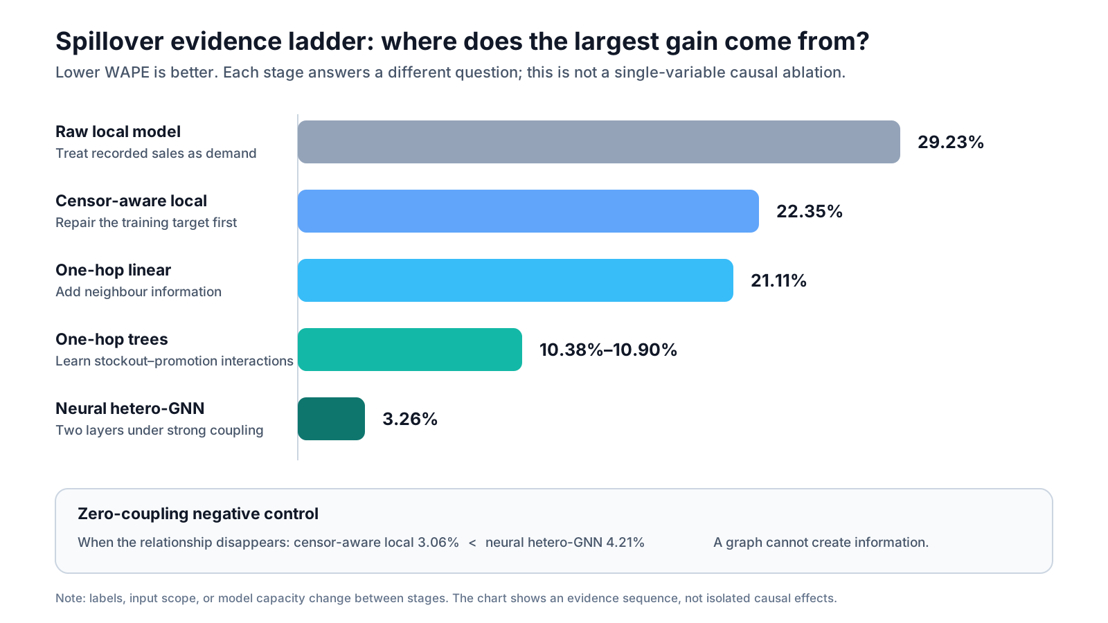
Adjacent stages do not all differ by one variable: labels, input scope, or model capacity change at different points. The figure is an evidence sequence, not a causal decomposition of every percentage-point gain.
5.3 Where Does Graph Value Appear? #
The coupling sweep turns “does the graph help?” from a binary question into a continuous one. When both cannibalization and spillover are zero, the analytical two-hop reference is 0.04 percentage points worse than the local model. Under the strong-coupling setting used in the main experiment, it leads by about 9.99 points. The gap grows with the share of transferred unmet demand and the intensity of promotional competition. Graph value therefore follows business coupling strength, not store count or the visual appearance of a network.
Store-level results follow the same pattern. Cross-warehouse hubs combine neighbour promotions with shocks from another warehouse, so they benefit most from upstream and spatial information. Stores dominated by their own stockouts first benefit from observation repair. Same-warehouse or weakly coupled stores often receive most of the available gain from a one-hop wide table. A production system therefore need not force one model on the whole network; it can tier models by store role and exposure to shocks.
Parameter sharing here means more than pooling ten stores into a larger sample. In the controlled network, well-stocked cross-warehouse hubs reveal complete spillover peaks, while inventory caps hide latent demand at constrained neighbours. One hypothesis to test is that a graph model can learn a shared relation rule where the signal remains visible and reuse it across edges of the same type. The experiment imposes that sharing mechanism; it does not prove that the same transfer occurs in real networks, which still requires validation across stores and time periods.
Readers usually care less about the network-wide champion than about which case resembles their own store. The table reports overall WAPE across the full test period for each representative position. Values in the one-hop column always follow the order Prophet, LightGBM, and XGBoost.
| Store role | Uncensored local | One-hop WAPE: Prophet / LightGBM / XGBoost | Neural heterogeneous GNN | Interpretation |
|---|---|---|---|---|
| Eastern cross-warehouse hub | 18.43% | 6.25% / 4.60% / 4.09% | 3.24% | Numerically lower, but the gap is below one point and is treated as an approximate tie. |
| Central cross-warehouse hub | 20.75% | 9.33% / 5.38% / 5.14% | 5.23% | XGBoost and the GNN are effectively tied; no clear graph increment appears. |
| Central flank store | 6.52% | 8.07% / 7.18% / 6.58% | 4.23% | A descriptive gap remains, but the small sample does not establish a stable ranking. |
| Western same-warehouse store | 12.54% | 9.02% / 3.86% / 4.25% | 4.01% | LightGBM and the GNN are approximately tied, leaving little reason to deploy the GNN. |
Prophet again shows that relational information does not belong to one model family. One-hop neighbour state substantially improves both cross-warehouse hubs even within an additive forecasting framework. Prophet still trails the trees, however, suggesting that these stores need conditional interactions as well as more fields. Comparing LightGBM with XGBoost also prevents the tree-model conclusion from depending on one implementation; LightGBM produces the lowest error at the western same-warehouse store.
No stable ordering works for every store. The best one-hop model and neural heterogeneous GNN are approximate ties at the eastern hub, central hub, and western same-warehouse store. The central flank shows a larger descriptive gap, but each store has only about 27 test days. Network-level results establish a direction; store-level results mainly identify what to test next.
Structural accuracy still cannot be translated directly into business return. The complete store matrix, peak dates, and feature importance remain in the experimental report. Inventory cost, service levels, and transfer constraints belong to the decision layer.
5.4 How Does Input Distortion Destroy Structural Gains? #
A relational model needs more than the existence of a field; the field must be timely and accurate. The stress tests use the analytical two-hop reference that closely matches the generator so that corrupted signals can be traced directly. They do not imply that every neural GNN would follow the same curve.
| Stress condition | Overall WAPE | Spillover WAPE | Meaning |
|---|---|---|---|
| Complete inputs | 3.79% | 3.95% | Mechanism reference under controlled conditions. |
| 30% of stockout flags missing | 12.10% | 22.49% | The structural gain nearly disappears when a key gate is absent. |
| Warehouse state delayed by one day | 12.46% | 20.39% | Correct but stale state cannot explain current spillover. |
| Single-node fault injection | Neighbour error expands sharply | Experimental circuit breaker reduces the radius | Graphs propagate bad signals; the breaker remains a test design. |
The node-fault experiment shows that bad data can travel to healthy stores. Removing the faulty node’s edges and falling back to a local model reduces the blast radius, but this is an experimental setting rather than a production-proven universal design. The same fault has not been injected identically into every candidate model, so the result does not establish that trees are inherently safer.
For example, after one central store receives tenfold promotion and sales spikes, WAPE at two one-hop neighbours rises from 5.68% and 2.91% to 48.03% and 43.54%. Unconnected clusters show no incremental error. The experimental circuit breaker lowers the two neighbours to 15.21% and 10.33%. It clearly limits the damage, but it does not restore clean-input performance. A breaker does not “solve” bad data; it keeps the error observable and allows the system to degrade locally.
5.5 How Do Methods Map to Tools? #
Tools solve implementation and engineering-abstraction problems; they cannot repair a missing information set. The current experiments map methods to tools as follows:
| Method role | Tool or solver | Purpose in the evidence chain |
|---|---|---|
| Linear ablations and analytical references | NumPy / SciPy | Hold capacity steady while testing observations, samples, and information. |
| Additive time-series model | Prophet | Test how a classical forecaster absorbs neighbour regressors. |
| Nonlinear neighbourhood wide table | LightGBM / XGBoost | Provide mature, expressive tabular baselines. |
| Neural heterogeneous GNN | NumPy / manual backpropagation and Adam | Learn multi-hop messages across different relation types. |
Historical Darts and LibCity timings from different environments are no longer mixed into the current comparison. Framework startup, compilation, and abstraction differ, so runtime is not an algorithm ranking. Information scope, interaction capacity, and operating responsibility should be compared first.
Tool choice should therefore begin with what the organization can already operate: a stable time-series feature pipeline, a mature wide-table training platform, or graph infrastructure capable of dynamic topology, node monitoring, and fault isolation. The same offline gain can imply very different deployment costs for different teams.
5.6 External Checks on Public Retail Data #
The final experiment uses ten-store panels from three public datasets to ask whether the controlled conclusions transfer. This is a boundary check, not another championship table.
I did not randomly split millions of item-level records. I first aggregated them into store-day panels, reserved the end of each timeline for testing, and estimated correlation weights from the training period only. Sales were rescaled by a constant to keep the numerical range convenient across solvers; scaling targets and predictions together does not change WAPE.
| Panel | Ten-store sample and evaluation summary | Graph construction |
|---|---|---|
| FreshRetailNet-50K[5] | Ten front warehouses and five products; 62 training / 28 test days, with a demand proxy reconstructed from stockout records. | Positive training-period correlation edges |
| Corporación Favorita[6] | Ten stores across three cities; 50 training / 21 test days, evaluated on observed sales. | Positive training-period correlations within each city |
| Walmart M5[7] | Ten stores across three states, using FOODS_1; 337 training / 28 test days, evaluated on observed sales. | Equal-weight edges within each state |
The full sampling rules, input fields, and target definitions are documented in the experimental report.
This processing puts three datasets with different scales and formats onto a common ten-store, daily unit of observation. It does not make their evidence equivalent: FreshRetailNet uses an author-constructed demand proxy, whereas the other two panels evaluate observed sales. Scores therefore compare models only within a panel, not dataset difficulty or mechanism strength across rows. The M5 periodic term and promotion proxy are constructed from dates and SNAP; they are not observed promotion fields supplied by the original data.
None of the three public panels provides the same upstream warehouse operating state—normal, congested, or disrupted—available at the forecast cutoff in the controlled experiment. They therefore cannot directly supply the same semantically defined input along a warehouse-to-store edge. FreshRetailNet includes stockout duration, but that is a store-side stockout record, not a warehouse operating state; the other two datasets lack a corresponding field. Treating sales-correlation or geographic proxies as observed warehouse-state chains would turn modelling assumptions into facts. The public panels therefore use a graph-aggregated ridge model, which feeds fixed graph summaries into ridge regression, rather than the neural heterogeneous GNN. It tests whether fixed relational summaries explain residual error with the available fields; it does not reproduce the controlled neural-GNN experiment.
The final column below is the graph-aggregated model’s WAPE difference from the best non-graph model.
| Public panel | Local baseline | Best non-graph model | Graph-aggregated ridge model | Difference |
|---|---|---|---|---|
| FreshRetailNet-50K | 26.74% | 26.74% (local) | 42.50% | +15.76 |
| Corporación Favorita | 13.23% | 12.11% (one-hop XGBoost) | 12.99% | +0.88 |
| Walmart M5 | 15.53% | 13.95% (one-hop linear) | 15.56% | +1.61 |
The FreshRetailNet local model still has a -24.9% bias despite leading the panel. Deleting stockout training days raises WAPE from 26.74% to 31.04%, so a cleaning rule that works in the controlled setting must be revalidated on real records.
The three rows reveal three possible roles for graph structure. On FreshRetailNet, the graph-aggregated ridge model is 15.76 percentage points worse than the local baseline, so training-period sales correlation does not produce a relationship that generalizes across the panel. The experiment does not isolate the cause. Correlation may create spurious edges, the demand proxy may change what the model needs to explain, or a 62-day training window aggregated to ten stores may limit generalization. On Favorita, the graph-aggregated model trails the best one-hop tree by only 0.88 points: regional aggregation may retain some shared signal, but it does not beat the tree’s treatment of promotion and payday nonlinearities. On M5, it nearly returns to the local baseline and trails the one-hop linear model by 1.61 points; grouping stores by state does not automatically create demand changes worth propagating.
Store-level results add one cautious qualification. The graph-aggregated ridge model records the lowest WAPE for the front warehouse labelled “Puxi boundary” in the FreshRetailNet panel (FRN_SH_06, 21.42%) and one California store (10.58%). That suggests relational summaries may help particular locations, but each store has a short test window and these are post-hoc comparisons across thirty stores. They do not establish a stable local advantage.
This section shows only that, with the available fields and graph-construction rules, fixed graph aggregation does not consistently beat non-graph baselines. It does not test the neural heterogeneous GNN or establish that real stores have no customer transfers. The next section explains why the controlled and public-data results answer different questions.
5.7 Why Do the Controlled Experiment and Public Data Give Different Answers? #
The different model rankings are not a contradiction. The controlled experiment specifies real cross-store coupling, timely supply states, and observable latent-demand truth. It asks whether a model can recover a known mechanism. The public-panel edges are constructed from sales correlations or regional membership, while latent demand is mostly unavailable. They ask whether the available evidence supports that mechanism in the first place.
The experiments therefore form three layers. At the observation layer, an uncorrected stockout label gives a complex model biased evidence to learn. At the information layer, timely one-hop neighbourhood states already improve Prophet and tree models substantially. At the structural layer, multi-hop message passing can add value only when real coupling leaves a stable cross-store residual. If any layer is missing, extra hops and model complexity may merely amplify a false assumption.
The result is not one champion for every retail network, but an order of judgment: repair observations, test cross-store information, and only then add structural complexity. Chapter 5 has explained what the evidence means; Chapter 6 turns that evidence into safer engineering choices.
5.8 Limitations and Next Steps #
What remains unidentified? The experiments lack a single promotion-by-stockout interaction control and matched-input multilayer perceptron and one-layer GNN baselines. They therefore cannot isolate the interaction’s contribution or separate continuous nonlinearity from graph structure. Three small comparisons could narrow those gaps: compare an MLP and one-layer GNN on matched inputs, add only the “neighbour promotion × neighbour stockout” feature to the linear baseline, and compare these results with the existing two-layer GNN. The coupling sweep also relies mainly on the analytical two-hop reference, and the stress tests do not inject identical faults into one-hop trees; the current evidence therefore cannot establish whether graph models are generally more fragile.
6. From Offline Evidence to Model Choice and Safe Execution #
Chapter 5 has interpreted the evidence. This chapter turns to production choices: how forecasts can support decisions without crossing inventory, authorization, and execution-safety boundaries.
6.1 Separate Forecasting from Execution #
Statistical models optimize an error-prone conditional expectation. Inventory, finance, and fulfilment systems maintain hard constraints that must never be violated. Even a graph model that is accurate on most days cannot guarantee that one transfer will not create negative inventory, consume stock reserved for online orders, or produce duplicate transfers after a network retry. Probabilistic forecasting and deterministic execution belong to different mathematical worlds.
| System layer | Main responsibility | Candidate techniques |
|---|---|---|
| Observation and cleaning | Detect closures and inventory censoring; repair training labels | Stockout filtering, censored likelihoods, data-quality rules |
| Forecasting | Estimate future latent demand and uncertainty | Local models, neighbourhood-feature tree models, heterogeneous graph models |
| Decision | Choose actions under cost and service constraints | Newsvendor models, operations research, business policy |
| Execution | Enforce inventory, authorization, idempotency, and recovery rules | State guards, workflows, transactions, audit trails |
| Monitoring | Track latency, drift, node anomalies, and condition-specific bias | Aggregate error, directional bias, quality alerts, and fallback policies |
Detecting a constrained warehouse and forecasting extra traffic at a cross-warehouse hub does not authorize an automatic transfer from another store. Source inventory may already be reserved, a vehicle may not meet its minimum load, or the destination’s receiving window may be full. The execution system must still check authorization and use transactions and idempotency keys to ensure that one request executes once. A forecast is an input to a decision; lower error cannot replace business safeguards.
6.2 Three Production Gates #
The controlled experiment assumes accurate, timely inputs and a stable topology. Real retail systems weaken each assumption.
- Phantom inventory and data latency. Shrinkage, theft, missed scans, and misplaced stock can leave book inventory above shelf availability. Warehouse congestion and transport delays may also arrive after the forecast job finishes. When a key state is unavailable at inference time, two-hop propagation can use only a missing or stale signal. The missing-stockout and delayed-state tests in Section 5.4 are controlled approximations of this problem.
- Unobserved factors and incorrect spatial edges. Roadworks, weather, competitor promotions, school holidays, and catchment changes affect traffic but may never enter company data. Proximity only permits two stores to exchange information; it does not prove a stable causal effect. A model can memorize a temporary common movement as a false edge, so topology needs out-of-time validation rather than one-off correlation-based construction.
- Fault propagation and dynamic topology. Independent store models naturally contain a fault. A graph model can pass corrupted input to neighbouring nodes. Openings, refurbishments, warehouse reassignments, and temporary dark stores also change nodes and edges. Production therefore needs node anomaly detection, edge-level circuit breakers, local-model fallback, and topology versioning.
Scale changes the problem as well. The experiment contains ten relatively homogeneous stores and one abstract product, while a live network may contain thousands of store formats and tens of thousands of stock-keeping units (SKUs). Expanding proximity, supply, and substitution together raises sampling, memory, and alignment costs; deep propagation can also over-smooth local differences. A graph decision must therefore account for modelling grain, network scale, and maintenance cost.
6.3 Choose Models Through an Evidence Ladder #
An engineering team can proceed in this order:
- Check whether inventory censored observed sales. If the training label confuses “could not sell” with “no one wanted to buy,” repair observation quality first.
- Confirm that cross-node signals exist by the inference cutoff. Promotion schedules, neighbour sales, and warehouse states must use the versions actually available at prediction time.
- Build a strong neighbourhood-table baseline that can express nonlinear interactions. This tests whether the existing tabular pipeline and a mature tree model can capture most relational value.
- Compare graph-neural-network gains only at important stores and during shocks. A lower network average does not mean every store needs the same model.
- Run like-for-like stress tests before deployment. Apply the same missingness, delay, and corruption to each candidate model and define circuit-breaker and fallback conditions in advance.
This sequence does not assume that any model family must win. Stores dominated by censored local sales and stable operations can remain on local models. When nonlinear neighbourhood interactions matter but fit a stable wide table, a mature tree model is often the lower-cost candidate. A graph neural network enters production evaluation only when multi-hop relationships add stable value and the organization can support the required data quality, node monitoring, and fault isolation.
6.4 Move Beyond Average Error #
A local model trained directly on inventory-censored sales has a directional bias of -13.87% against latent demand, worsening to -29.23% when customers transfer from stocked-out neighbours. The negative sign means that the system persistently underestimates demand rather than making errors that merely vary in direction from day to day. If a company feeds such forecasts directly into replenishment, it can create a self-reinforcing chain: a stockout lowers observed sales, the system then lowers its demand forecast and replenishment quantity, and the next stockout becomes more likely. Evaluation must therefore examine persistent over- or underforecasting, important operating conditions and stores, and whether required inputs arrive reliably—not only one network-wide average error.
A mature system is not one with an ever-deeper graph. It is one in which every relationship can be tested, invalidated, and withdrawn: strong local models carry local patterns, while a relational component corrects only the cross-store residuals that demonstrably remain. Forecasts remain evidence for decisions and stay subordinate to inventory, cost, authorization, transaction, and state-machine constraints.
Conclusion: Using a Graph Perspective Does Not Require Deploying a Graph Model #
The store that opened this article with an unexpected rush reminds us that demand can depend on relationships with nearby entities, but seeing those relationships does not require deploying a graph model. A reliable choice first corrects observations, verifies which information is available at forecast time, and then tests whether a model adds stable value. Simple models may win; graph models are worth considering only when their relationships are credible, their data timely, and their risks manageable, and no forecast should bypass inventory, cost, authorization, or execution safeguards.
Continue reading and reproduce the experiments: See the retail-gnn-demand-forecast GitHub repository for the implementation, data loaders, and experiment entry points. The full experimental report contains model configurations, store-level results, stress tests, and run records. When reproducing the public panels, verify the sampling, graph construction, and target definitions in Section 5.6 together with the scores.
References #
[1] Gilmer, J., et al. Neural Message Passing for Quantum Chemistry. Proceedings of the 34th International Conference on Machine Learning, 2017. https://proceedings.mlr.press/v70/gilmer17a.html
[2] Kipf, T. N., & Welling, M. Semi-Supervised Classification with Graph Convolutional Networks. International Conference on Learning Representations, 2017. https://arxiv.org/abs/1609.02907
[3] Hamilton, W. L., Ying, R., & Leskovec, J. Inductive Representation Learning on Large Graphs. Advances in Neural Information Processing Systems, 2017. https://proceedings.neurips.cc/paper/2017/hash/5dd9db5e033da9c6fb5ba83c7a7ebea9-Abstract.html
[4] Veličković, P., et al. Graph Attention Networks. International Conference on Learning Representations, 2018. https://arxiv.org/abs/1710.10903
[5] Dingdong Inc. FreshRetailNet-50K: A Stockout-Annotated Censored Demand Dataset for Latent Demand Recovery and Forecasting in Fresh Retail. arXiv:2505.16319, 2025. https://huggingface.co/datasets/Dingdong-Inc/FreshRetailNet-50K
[6] Corporación Favorita. Corporación Favorita Grocery Sales Forecasting. Kaggle, 2017. https://www.kaggle.com/competitions/favorita-grocery-sales-forecasting
[7] Makridakis, S., Spiliotis, E., & Assimakopoulos, V. The M5 Accuracy Competition: Results, Findings, and Conclusions. International Journal of Forecasting, 2022. https://doi.org/10.1016/j.ijforecast.2021.11.013